Multi-Output Aerodynamic Prediction with Physics-Informed Neural Networks
A physics-informed neural network that predicts an airfoil's lift, drag, and moment in a millisecond, trained on 52,480 NASA CFD simulations. The full network runs live below, in your browser, on TensorFlow.js. Drag the shape and watch the aerodynamics update in real time.
CFD is the truth, but it is slow
Every wing, blade, and UAV begins with one question: for this shape, at this speed and angle, what are the lift, drag, and moment? Computational fluid dynamics answers it accurately by solving the governing equations on a mesh, but a single high-fidelity run can take hours.
Design optimization needs that answer thousands of times, across a whole space of shapes and flow conditions. At CFD speed, that loop is impractical. The goal of this project was a surrogate: a model that keeps CFD-level accuracy while returning an answer instantly, so a designer can explore the whole space interactively.
READ MORE · METHODCONTEXT, GAP, AND METHOD
The paper asks a practical design question: can one surrogate remain accurate across geometry, Reynolds number, Mach number, and angle of attack, including stall and airfoils excluded from training? Its answer is a geometry-aware, physics-informed neural network trained on high-fidelity CFD.
Why a new surrogate?
High-fidelity CFD resolves the governing flow equations and is the reference used here, but repeated meshing and solution make it too expensive for multidisciplinary design optimization. Conventional response surfaces and ordinary neural networks are fast, yet they can interpolate without learning the correct aerodynamic trends, particularly near sparse regions, stall, and a new geometry.
The related work reviewed in the paper spans data-driven MLP and CNN surrogates, physics-informed neural networks, generative airfoil design, and compact parameterizations such as CST. The unresolved issue is not only test-set accuracy; it is whether the model remains interpretable and physically plausible when the airfoil itself was never present during training.
That distinction changes the research target. A random train/test split can reward memorization because neighboring operating points from the same airfoil appear on both sides. The method therefore treats geometry as a first-class variable and measures success on entire shapes removed from optimization. It also predicts Cl, Cd, and Cm together because an efficient design cannot be judged by lift alone; drag determines efficiency and pitching moment determines trim and stability.
What this work contributes
Compact geometry
Every coordinate file is converted into upper and lower CST coefficients, giving the network a continuous shape description instead of an arbitrary cloud of points.
Derivative features
The Fast Derivative Layer exposes how learned features change with angle of attack, then fuses that sensitivity into the shared representation.
Physics curriculum
Data fit, derivative constraints, drag-polar structure, hard-case sampling, and tail losses are introduced in stages rather than optimized all at once.
How it fits into a design loop
A conventional optimization loop proposes a geometry, builds a mesh, runs the flow solver, extracts coefficients, and repeats. Here, CFD is paid for once when constructing PALMO. Each later candidate is normalized, encoded by CST, evaluated by the network, and screened in milliseconds. Promising candidates can still be returned to CFD for confirmation, turning the surrogate into a fast search layer rather than an unqualified replacement for simulation.
The paper's method is deliberately coefficient-focused. It does not reconstruct pressure or velocity fields, so it is far lighter than a field surrogate and directly matches the quantities required by many conceptual and preliminary design studies.
Core distinction: this is not a flow-field solver and it does not replace CFD outside its trained design family. It is a coefficient surrogate for fast exploration inside a documented aerodynamic envelope.
52,480 CFD simulations from NASA
The model learns from PALMO, a high-fidelity dataset generated at NASA Ames with the OVERFLOW solver and Spalart-Allmaras turbulence closure.
It covers the NACA 4-series (from 0006 to 4424) across an unusually broad envelope: Mach 0.25 to 0.90, Reynolds 75k to 8M, and angle of attack −20° to +20°. Twelve airfoils were used for training; four were held out entirely as a strictly unseen test of generalization.
READ MORE · DATA52,480 CFD CASES
PALMO is treated as the aerodynamic ground truth. It was produced at NASA Ames with OVERFLOW, using second-order temporal accuracy, fourth-order spatial differencing, and the Spalart-Allmaras turbulence model.
| AXIS | VALUES USED IN THE PAPER | ROLE |
|---|---|---|
| Geometry | 16 NACA 4-series airfoils, 0006 through 4424 | Shape generalization |
| Mach | 0.25, 0.35, 0.45, 0.55, 0.65, 0.70, 0.75, 0.80, 0.85, 0.90 | Subsonic to transonic effects |
| Reynolds | 75k, 125k, 250k, 500k, 1M, 2M, 4M, 8M | Viscous-scale variation |
| AoA | −20° to +20° at integer increments | Linear range, stall, and reverse loading |
| Targets | Lift Cl, drag Cd, pitching moment Cm | Coupled aerodynamic response |
A split that actually tests a new shape
Twelve airfoils supply the development data. Their cases are divided 80/20 into training and held-out test samples. Four complete geometries, NACA 4421, 3418, 4415, and 3415, are removed before training and used only for the unseen-airfoil evaluation. This is stricter than randomly hiding operating points from a shape already known to the network.
Seen test
New Mach, Reynolds, and AoA combinations drawn from airfoil families represented in training.
Strictly unseen
All operating points belong to four geometries whose CST vectors were never used to fit the network.
Explore the simulation lattice
The lattice is balanced by construction: every geometry is sampled at the same flow conditions and integer angles. This makes cross-geometry comparisons cleaner, while the 41-point AoA sweep supplies enough ordered samples to learn the attached-flow slope, nonlinear transition, and post-stall behavior. Multiplying 16 × 10 × 8 × 41 gives the reported 52,480 simulations.
Deployment envelope: the paper trains on the complete −20° to +20° database. The browser demo intentionally presents −10° to +15°, the more useful interactive design range requested for this page. Reynolds and Mach retain the paper's full ranges.
An airfoil in a handful of numbers
A neural network cannot ingest a raw list of surface points. The shape is encoded with the Class-Shape Transformation (CST): a class function fixes the round nose and sharp tail, and a small set of Bernstein weights bend the surface between them.
Eighteen coefficients describe an entire airfoil, smoothly and physically. That compactness is what lets the model generalize to shapes it has never seen. The animation shows the Bernstein basis blending into the final curve.
READ MORE · CST FITFROM COORDINATES TO 18 FEATURES
CST separates the universal topology of an airfoil from the coefficients that describe a particular shape. The same differentiable equation is used for the paper preprocessing and for the draggable browser geometry.
The class exponents create a rounded leading edge and a finite, sharp trailing edge. The shape function is an order-7 Bernstein expansion, so each surface has eight weights. Upper and lower trailing-edge offsets add two more inputs, producing the 18 geometry variables used by the model.
By tying the first upper coefficient to the sign-reversed first lower coefficient, the fit retains the rounded CST nose and a differentiable surface transition. This is the key idea behind making sparse coordinate files usable as smooth neural-network inputs without losing leading-edge physics.
Coordinate preparation and robust fitting
- Move the leading edge to the origin, align the chord, normalize it to unit length, and identify the trailing edge.
- Split the coordinate loop into upper and lower surfaces and resample them consistently.
- Fit the two Bernstein expansions independently with robust least squares and a soft-L1 residual.
- Couple the first upper and lower coefficients with opposite sign, preserving leading-edge symmetry and tangent continuity.
- Reconstruct the profile and reject perturbations that create surface crossing, excessive thickness or camber, or an invalid nose and trailing edge.
The robust objective is important near the leading and trailing edges, where coordinate ordering, duplicate points, and small measurement offsets can otherwise dominate an ordinary least-squares fit. Soft-L1 behaves quadratically for normal residuals but reduces the influence of isolated bad points. After fitting, reconstruction error and geometric validity are checked in physical coordinates before the coefficients enter the learning dataset.
8 upper
Bernstein weights describe suction-side curvature from nose to trailing edge.
8 lower
A separate expansion represents the pressure side without forcing symmetry.
2 offsets
Upper and lower Δz terms retain the measured trailing-edge closure.
Why the live shape now looks correct: the visible curve is densely evaluated from the CST equation, not connected through a few draggable points. Handles only perturb nearby valid CST coefficients, while the reconstructed surface remains smooth at the nose and along the chord.
Physics, built into the wiring
The inputs — Reynolds, Mach, angle of attack, and the CST geometry — pass through a shared encoder, then split into three heads for lift, drag, and moment.
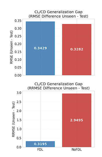
Two ideas make it physics-informed. The angle of attack gets a frequency encoding so the network can represent sharp, periodic effects like stall. And a Fast Derivative Layer computes ∂(hidden)/∂α and injects those sensitivities back into the features, so physical reasoning lives inside the network, not just in the loss. That one change cut the error on unseen airfoils by nearly ten times.
READ MORE · NETWORK23 INPUTS, FDL, 3 HEADS
The model combines physical state, compact geometry, a frequency representation of angle of attack, and learned angle sensitivities. Three specialized output heads then share the same aerodynamic representation.
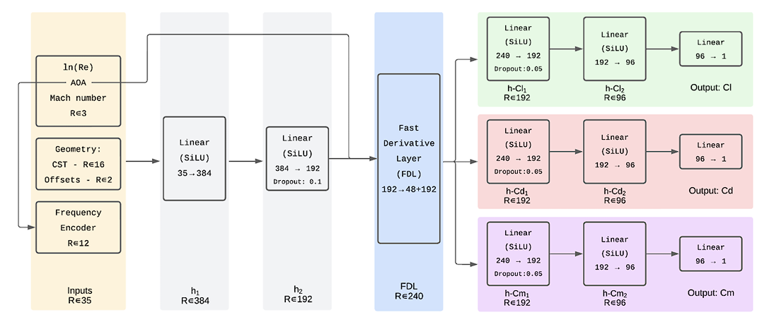
From 23 physical values to three coefficients
| STAGE | DIMENSION / OPERATION | PURPOSE |
|---|---|---|
| Raw input | ln(Re), AoA, Mach + 18 CST geometry values = 23 | One vector describes both flow and shape. |
| AoA encoding | 6 bands, 12 sine/cosine channels; 23 → 35 | Resolves nonlinear and rapidly changing angular behavior. |
| Encoder | 35 → 384 → 192, SiLU + dropout | Learns a shared aerodynamic latent state. |
| FDL | First 48 hidden sensitivities ∂h/∂α; 192 + 48 → 240 | Makes angle response available as a feature. |
| Heads | Three branches, 240 → 192 → 96 → 1 | Separate Cl, Cd, and Cm specialization. |
Fast Derivative Layer
During gradient-enabled training, automatic differentiation calculates the derivative of the first 48 latent features with respect to AoA. The derivatives are scaled by 0.05 and concatenated with the 192-dimensional encoder output. This differs from a standard PINN that uses derivatives only as a penalty: here the sensitivity becomes part of the representation consumed by every output head.
For exported inference, the derivative branch is zero-filled, matching the original notebook implementation. Its training influence is still embedded in the learned encoder and head weights. This detail matters because the browser must reproduce the saved model, not silently invent a different inference graph.
Stable targets and hard cases
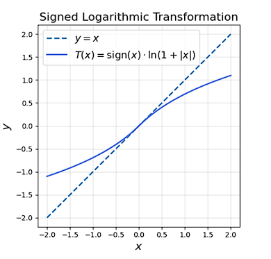
Signed-log transforms preserve the direction of lift and moment while compressing extremes. Drag uses log1p because it is nonnegative, and the inverse path applies expm1 plus a nonnegative clamp. StandardScaler statistics are learned from training data only. A weighted sampler later gives higher probability to examples whose error exceeds the current mean, concentrating capacity on stall and other difficult regions.
The six-frequency AoA encoding is concatenated with, rather than substituted for, the physical angle. The raw coordinate preserves ordering and extrapolation direction, while sine and cosine channels give the MLP a richer basis for steep curvature near stall. The three heads share low-level flow and geometry information but can specialize their final layers for the very different scales and shapes of Cl, Cd, and Cm.
Taught the rules, not just the data
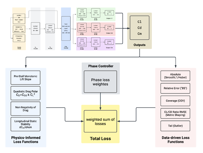
Fitting the data is not enough; the predictions must obey physics. Training ran as a multi-phase curriculum that slowly turns up physics-based penalties.
Three constraints are enforced softly: lift should rise with angle before stall (∂Cl/∂α > 0), the moment should keep the airfoil stable (∂Cm/∂α < 0), and drag must follow a proper polar (Cd ≈ Cd₀ + k·Cl²) and never go negative. This is what keeps the surrogate trustworthy where data is thin.
- Lift slope — ∂Cl/∂α > 0 before stall
- Stability — ∂Cm/∂α < 0
- Drag polar — Cd ≈ Cd₀ + k·Cl²
- Non-negative drag — Cd ≥ 0 always
- Hard-example mining — focus on the cases it gets wrong
READ MORE · TRAININGDATA, PHYSICS, TAILS
The objective is a controlled mixture of data accuracy and aerodynamic structure. Masks and gates restrict each physics rule to the regime where it is valid, so the optimizer does not force pre-stall behavior onto stalled or compressibility-dominated samples.
Physics terms
Pre-stall lift
Penalizes negative ∂Cl/∂α in the attached-flow window, with stall and Mach gating.
Static stability
Discourages positive ∂Cm/∂α where a stable pitching response is expected.
Drag polar
Encourages Cd = Cd₀ + kCl² locally, rather than fitting drag as an unrelated scalar.
Physical bounds
Prevents negative drag and suppresses implausible behavior using flow and geometry masks.
Data and robustness terms
The supervised core uses SmoothL1, which behaves quadratically around small errors and linearly for large residuals. Relative-error shaping balances coefficients with different scales. Coverage terms discourage systematic misses, a tail loss protects extreme cases, and a Cl/Cd ratio term improves the derived efficiency metric. The weighted hard-example sampler is activated only after the base map has stabilized.
Each rule is evaluated through a validity mask. For example, positive lift slope is a useful attached-flow prior but becomes incorrect beyond stall, and a simple quadratic drag polar is most defensible away from strong transonic effects. Mach, AoA, stall, and geometry gates therefore decide where a penalty contributes. This keeps “physics-informed” from becoming “physics-forced” in regimes where the simplified rule no longer applies.
| PHASE | FOCUS | WHAT CHANGES |
|---|---|---|
| 1 · Foundation | Data fit + physics | Physics weight 0.5; no tail loss, ratio polishing, or hard sampler. |
| 2 · Hard cases | Physics + tails | Physics weight 0.4; hard-example mining and tail protection are enabled. |
| 3 · Polish | Relative and efficiency accuracy | Physics weight 0.2; stronger Cl/Cd ratio and relative-error optimization. |
Training runs for 220 epochs with learning-rate warmup followed by cosine decay, checkpointing the best validation model. On an RTX 3090 the reported training time is under 30 minutes.
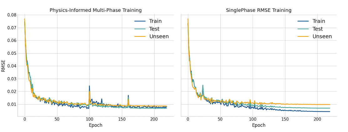
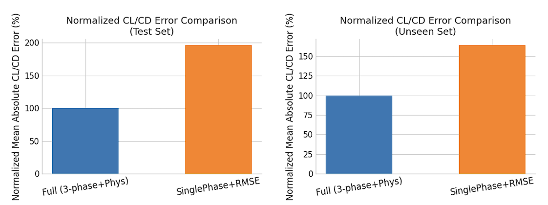
Why the order matters: enforcing every objective from epoch one makes gradients compete before the network has learned the basic CFD map. The staged schedule first establishes that map, then concentrates on physics, tails, and ratios.
CFD accuracy, at interactive speed
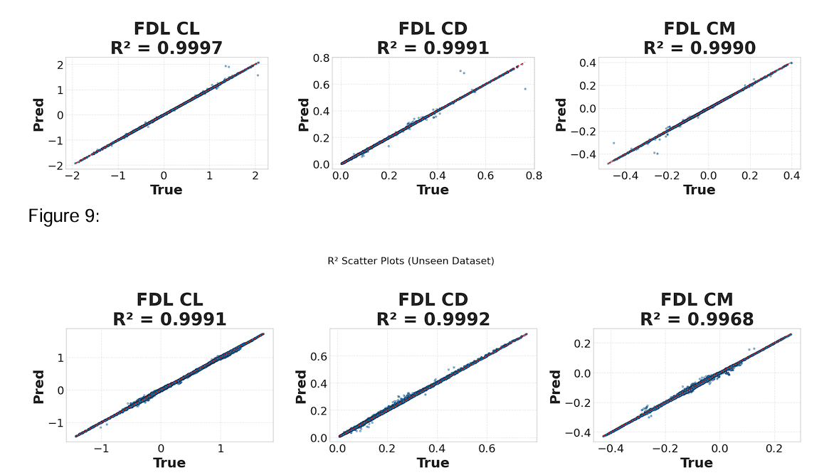
On the held-out test set the model reaches R² = 0.9997 for lift, 0.9991 for drag, and 0.9990 for moment.
The real test is the four airfoils it never saw during training. There it stays strong (R² ≈ 0.999 for lift and drag), which is exactly what the Fast Derivative Layer and the physics curriculum were built to protect. A prediction that used to cost hours of CFD now costs about a millisecond.
READ MORE · EVIDENCEEVIDENCE FROM THE PAPER
The evaluation checks more than one aggregate score: coefficient parity, complete angle sweeps, three-dimensional operating maps, ablations, an external surrogate comparison, symmetry, and a deliberately difficult out-of-family experiment.
| SPLIT | CL | CD | CM |
|---|---|---|---|
| Held-out test R² | 0.9997 | 0.9991 | 0.9990 |
| Held-out test RMSE | 0.0123 | 0.0043 | 0.0033 |
| Unseen-airfoil R² | 0.9991 | 0.9992 | 0.9968 |
| Unseen-airfoil RMSE | 0.0178 | 0.0040 | 0.0045 |
R² measures how much variation in the CFD outputs is explained, while RMSE preserves each coefficient's physical scale. Both are needed: a high R² can coexist with a practically important local error, and direct RMSE values are not comparable across coefficients without remembering that drag and moment are numerically smaller than lift.
Does it reproduce complete aerodynamic curves?
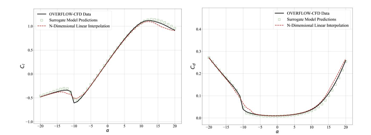
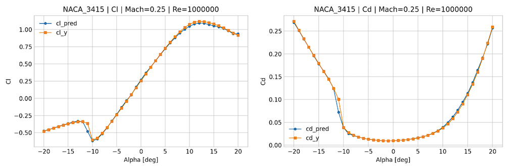
For the unseen NACA 3415 at Mach 0.25 and Re = 1M, the PINN follows PALMO across the full angle sweep, including the nonlinear transition and stall near −10°. The paper's NASA surrogate/interpolation baseline misses this behavior more clearly, illustrating why global R² alone is not sufficient.
Curve-level agreement tests continuity and ordering, not only isolated residuals. The lift curve should recover the linear slope and both stall branches; drag should stay positive and rise as loading grows; Cm should maintain a plausible stability trend; and Cl/Cd should peak in a localized efficient corridor rather than oscillate between adjacent angles.
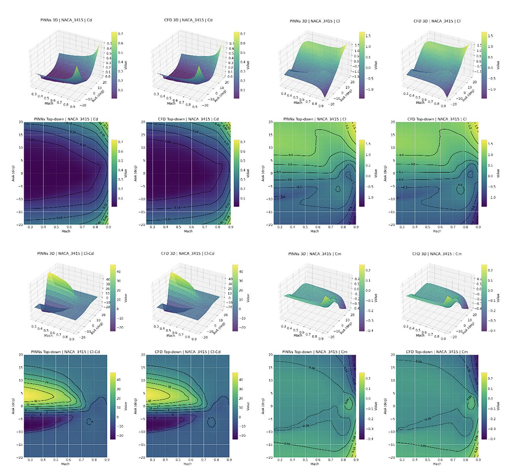
Maps over Mach and angle of attack
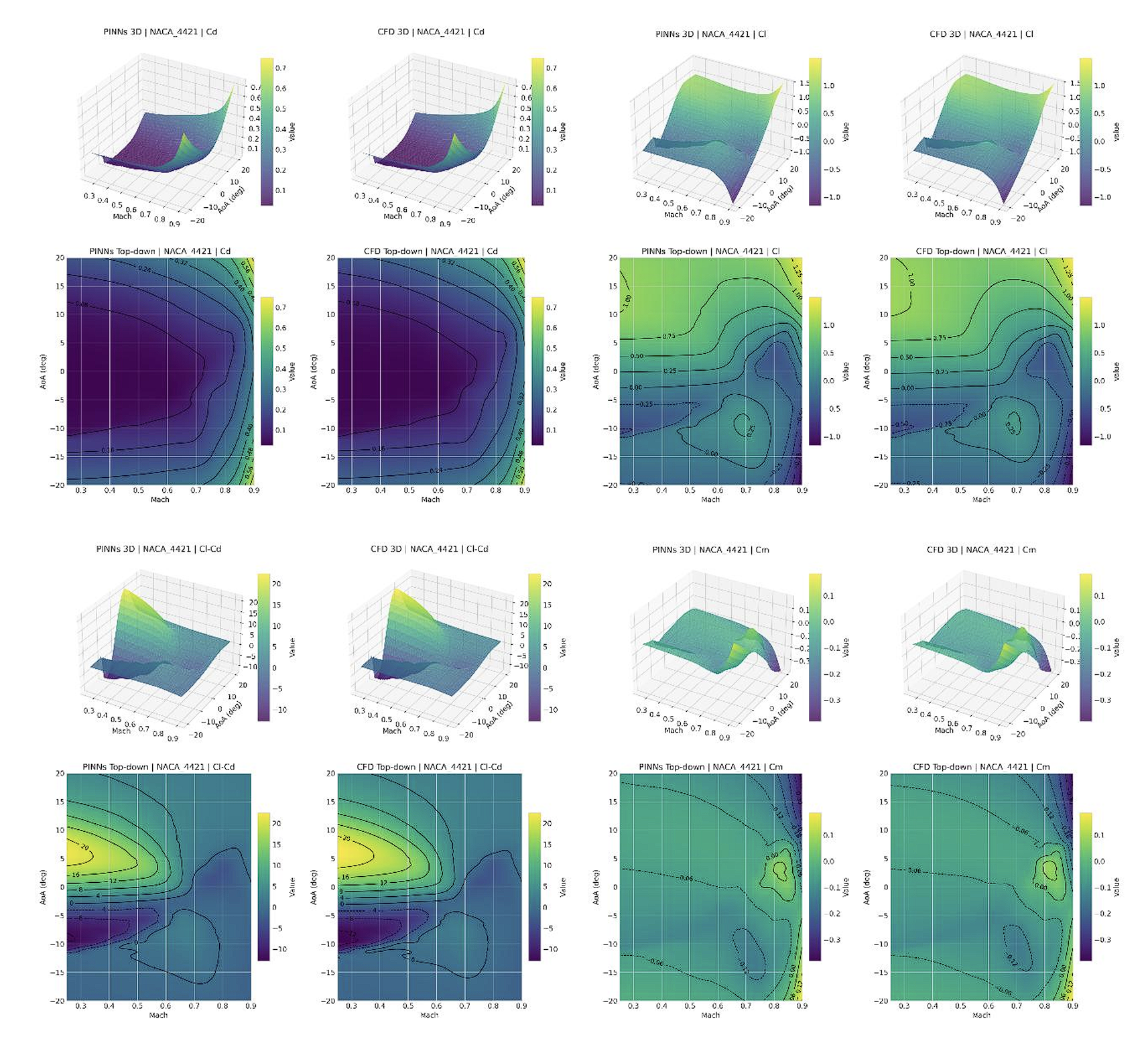
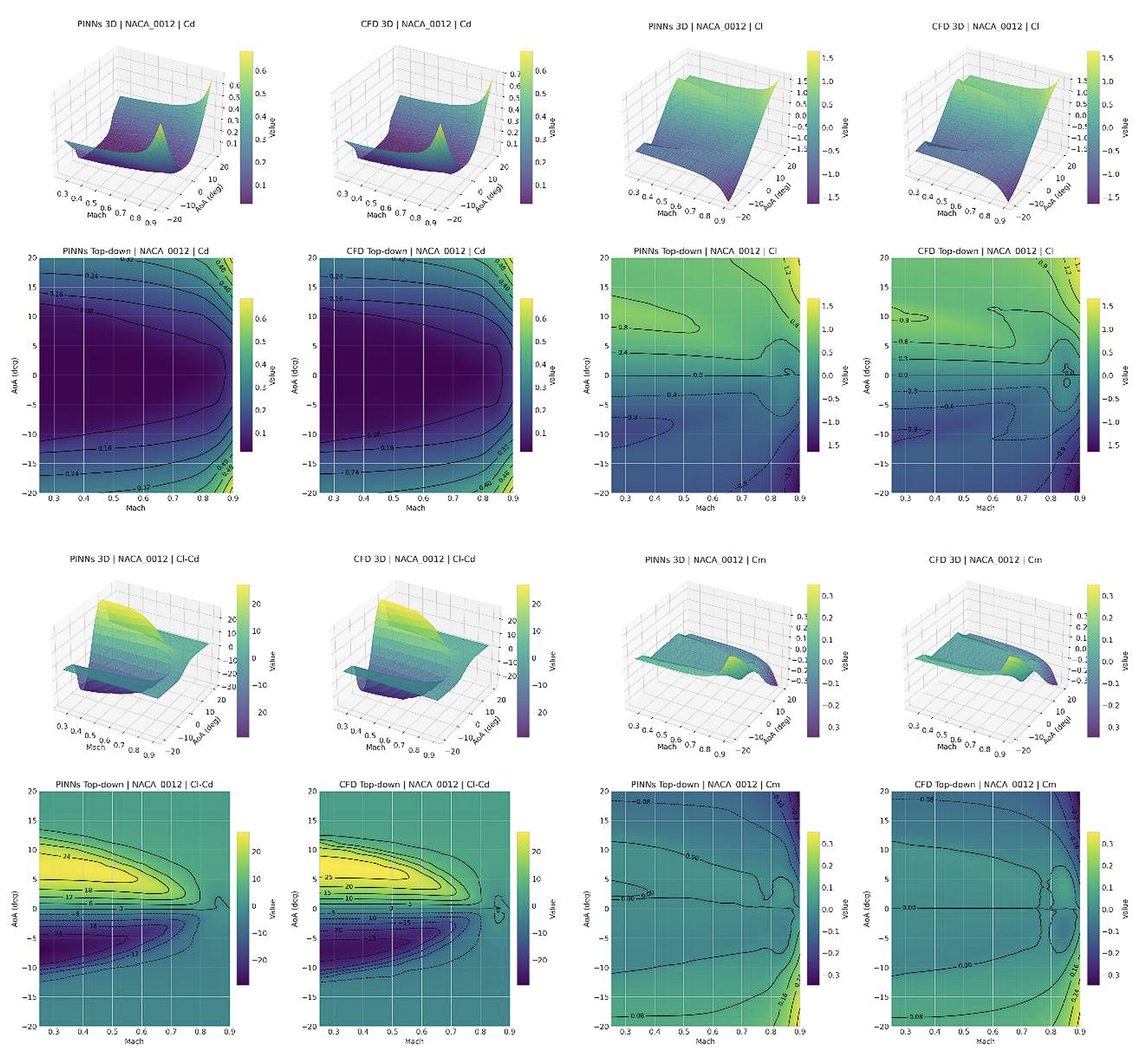
The surface and contour plots show that the network learns coupled aerodynamic structure rather than isolated point predictions. Lift grows through the attached-flow range and rolls off around stall; drag rises rapidly at high loading and compressibility; moment changes consistently with camber and stability; efficiency peaks in a bounded operating corridor. The symmetric NACA 0012 case also provides a useful reversal and near-zero-moment check.
What each ablation established
- FDL: removing hidden angle sensitivities sharply damages unseen-shape robustness.
- Three-phase curriculum: a single training phase produces a larger train-to-unseen gap and worse efficiency prediction.
- Signed-log and frequency features: target transforms and AoA encoding reduce drag error, especially at extreme angles.
- Physics losses: derivative and drag-polar constraints improve trends in sparse regions instead of merely improving pointwise averages.
Limitations and the failure study
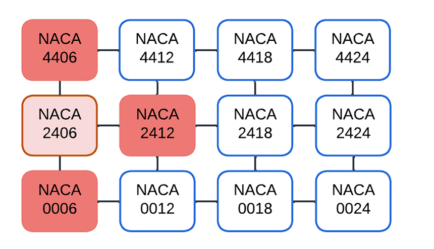
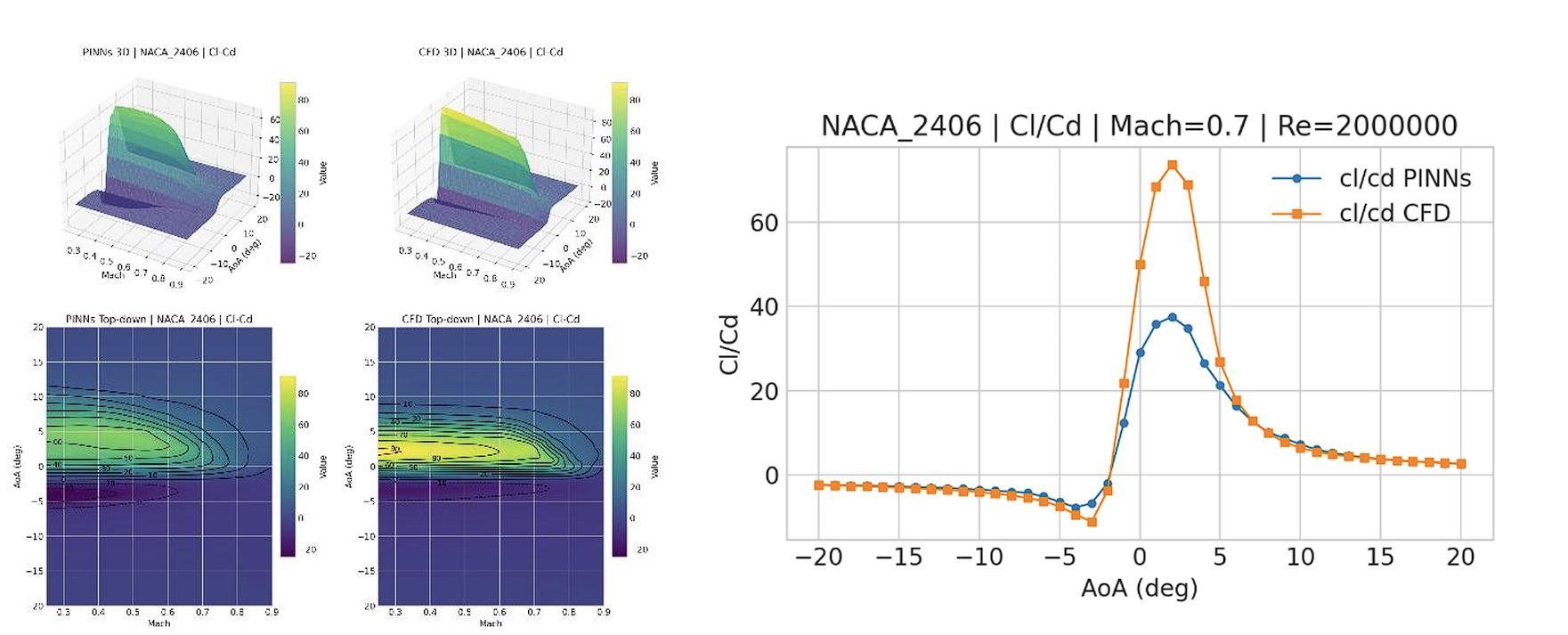
The model is intentionally scoped to the NACA 4-series distribution represented in PALMO. To test a more difficult geometric gap, the paper removes NACA 2406 and close variants from training. The network still identifies the broad stall pattern, but peak Cl and Cl/Cd become less accurate. That result sets an important boundary: physics guidance improves interpolation and nearby generalization, but it cannot replace representative CFD coverage.
This failure case is scientifically useful because it separates smooth response regularization from geometric knowledge. The derivative losses can teach how coefficients ought to vary with AoA, but they cannot infer an unobserved thin-airfoil response perfectly when nearby thickness and camber combinations are absent. A production system should therefore measure distance in standardized CST space, flag remote candidates, and route the most informative ones back to CFD.
Next steps from the paper: expand beyond NACA 4-series families, quantify predictive uncertainty, and use targeted data acquisition to add CFD cases where uncertainty or geometric distance is highest.
Design an airfoil, feel the aerodynamics
The exact trained network, running on TensorFlow.js. Drag the CST geometry, set the flow conditions, and compare the live prediction against PALMO CFD whenever the selected case exists in the training database.
READ MORE · LIVE MODELREAL WEIGHTS, CST, CFD OVERLAY
This is the exported trained surrogate, not a hand-written aerodynamic approximation. The page reconstructs the PyTorch layers and exact float32 checkpoint weights in TensorFlow.js, then applies the paper's feature order, scalers, frequency encoding, output transforms, and inverse transforms.
Geometry path
Preset coordinates are represented by the same 18D CST form. Dragging changes bounded CST parameters and reruns the validity guard before prediction.
Flow path
Mach 0.25–0.90, Reynolds 75k–8M, and AoA −10° to +15° stay inside the intended browser envelope.
Evidence path
For an unchanged database airfoil, the charts draw PALMO CFD beside the prediction. Once geometry is edited, only the model curve is shown.
Exact inference sequence
- Validate the edited CST vector and reconstruct a dense, non-intersecting airfoil surface.
- Build the 23 physical inputs in the notebook's original order, using ln(Re) and the saved training scalers.
- Append all 12 sine/cosine AoA features and evaluate the shared encoder plus the three trained heads.
- Undo standardization and signed-log transforms to recover physical Cl, Cd, and Cm.
- Repeat across the displayed AoA grid, then retrieve a PALMO reference only when geometry and flow conditions match a stored case.
Reading the plots correctly
The lift and efficiency panels are evaluated over every half degree in the displayed AoA range. The drag polar uses the same predictions with Cd on the horizontal axis and Cl vertically. Smooth strokes are only a visual interpolation between deterministic samples; the coefficient values are not randomized or filtered with synthetic noise.
When a preset exactly matches a PALMO geometry and database condition, the reference curve provides a direct CFD comparison. For a custom CST shape there is no CFD record to display, so the page labels it as prediction-only. Geometry guards limit thickness, camber, control-point movement, surface crossing, nose continuity, and trailing-edge closure, reducing extrapolation into obviously invalid airfoils.
The current white marker is the selected AoA, while the full line is a fresh batch evaluation at the chosen Mach, Reynolds number, and geometry. This makes local coefficient changes and global curve changes visible together. Because all output values come from one deterministic forward pass, moving a control does not inject measurement noise or randomly jitter the plot.
Scientific boundary: an interactive prediction is reliable only to the extent that its geometry and operating condition remain close to the PALMO/NACA 4-series domain. The demo exposes that boundary rather than presenting arbitrary shapes as CFD truth.
A wind tunnel that fits in a web page
Compact geometry, a physics-aware network, and a curriculum that teaches the laws add up to a surrogate you can actually design with: CFD-level answers, instantly, even on shapes it never trained on. Everything above ran the real weights, live.
READ MORE · CONCLUSION
The paper's central result is that compact CST geometry, latent angle derivatives, and staged physics-aware optimization can preserve near-CFD coefficient accuracy while cutting inference to interactive time. The unseen-airfoil tests show strong interpolation across the studied NACA family; the NACA 2406 stress test shows why training-envelope coverage still matters.
The proposed research direction is therefore not to abandon CFD, but to use it strategically: broaden the geometry families, attach uncertainty estimates to each prediction, and request new high-fidelity cases only where the surrogate is uncertain. That closes the loop between accurate simulation and rapid design exploration.